Tutorial for Spreadsheet Users

About This Tutorial

This tutorial is designed for business and enterprise users who will use Row Zero’s spreadsheet capabilities to analyze data and share insights. By the end of this tutorial, you will build an automatically refreshing spreadsheet with pivot tables and charts and then share it with others in your workspace.

In this tutorial, you will:

Import data from a shared data source into a workbook and configure a scheduled refresh to automatically refresh your data.
Create a pivot table and a chart to analyze your data.
Share your workbook with other users.

Prerequisites:

Spreadsheet proficiency: You will get the most out of this tutorial if you have some familiarity with spreadsheets, including basic knowledge of functions, pivot tables, and charts.
Shared data source: This guide assumes you have already created a data source or someone in your organization has shared one with you. If not, refer to our Tutorial for Query Writers to publish a data source first.

Note: This tutorial does not cover administration or integrations. For those topics, refer to our launch guides and documentation. This tutorial also does not cover writing queries or publishing data sources. For those topics, refer to our Tutorial for Query Writers.

Overview: What Is Row Zero?

Row Zero is a high-performance spreadsheet built for big data. While traditional spreadsheets struggle with large files, Row Zero enables you to analyze 10 million, 100 million, or even billion row datasets. It connects directly to your data warehouse, enabling you to access real-time datasets from the familiar interface of a spreadsheet.

To build effectively in Row Zero, it is important to understand two key concepts: workbooks and data sources.

Workbooks are spreadsheets that contain data, formulas, and/or visualizations. Workbooks support a variety of use cases, including modeling, analysis, and dashboards. You can import data from connections into your workbooks by directly querying connections or inserting data from a data source.

Data sources are published queries. They are used to manage governed “source of truth” datasets or to give less technical users direct access to live data without writing SQL.

When you log into Row Zero, your home page will look something like this:

New User Home Screen

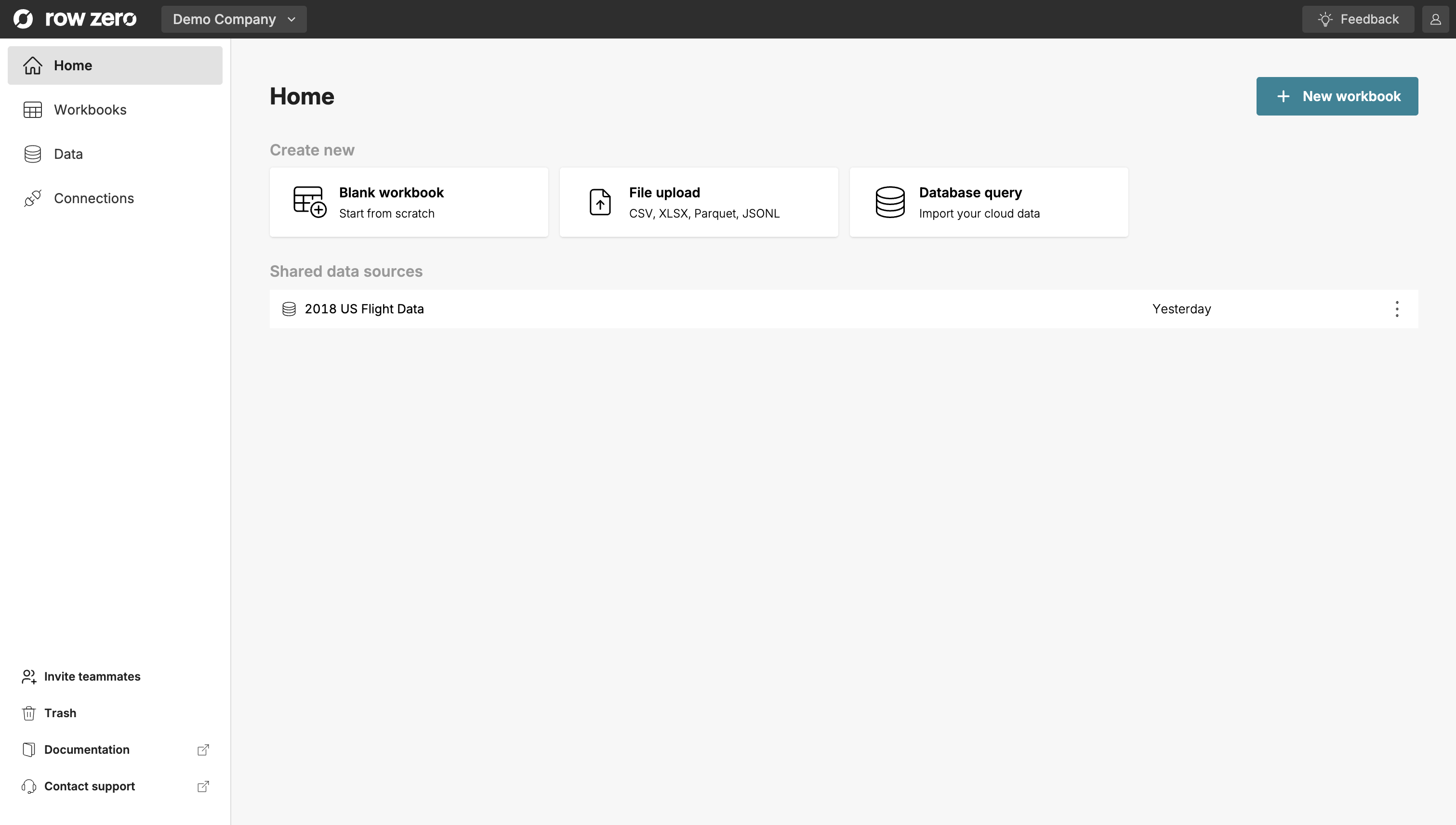
Use the menu on the left side to navigate to a new section:

Home: Once you've created workbooks or data sources (or others have shared them with you) this page will give you quick access to your most recent files.
Workbooks: A list of all workbooks you have created or that have been shared with you.
Data: The list of published data sources that you have created or that have been shared with you.
Connections: Where you manage your credentials and integrations for external data warehouses.

Create a Workbook

In this section, you’ll create your first workbook.

To create a new workbook, click Blank workbook from your home page.
Give your workbook a name by clicking Untitled Workbook at the top. Let’s name this workbook “Spreadsheet User Tutorial”.

If you’ve used a spreadsheet before, the UI should look familiar. On the toolbar, you’ll find zoom, formatting options, as well as shortcuts to create pivot tables, charts, filters, and conditional formatting.

You can navigate back to the home page any time by clicking the Row Zero icon in the top left corner.

Functions

Row Zero supports over 250 Excel and Google Sheets-compatible functions. Type a function into a cell to view a detailed description of its arguments and results. Additional function documenation and examples are in our documentation. You can also create custom functions using the Python code window.

Import Data From a Data Source

Row Zero supports several methods for importing data including uploading a file, querying a connection (e.g. Snowflake, Databricks, etc.), and inserting a data source. In this tutorial, you’ll import data from a data source published by your team.

Data sources are reusable, published queries. They are an easy way for your data team to give other users no-code access to live data.

Note: If your data team has not yet created or shared data sources, you can direct them to our Tutorial for Query Writers.

Import Data

To insert a data source into your workbook:

Click Data to open the Data side panel.
Select a data source from the data sources tab.
Select your Destination. If needed, enter values for any query variables to filter your data. By default, Row Zero will import all data source columns, but you can import just a subset by clicking Specific columns and selecting your desired columns. Both options are useful when the full data set is very large.
Click Insert data source. The data source will open in a new connected table.

A connected table is a type of data table. Data tables float on top of your worksheet and are anchored to the upper-left cell the data table covers. Connected tables include all the data from the imported dataset and have a scroll bar on the right side of the table. These tables are read-only, so data within the table cannot be overwritten.

You can navigate back to this side panel anytime by double clicking the connected table, or by right clicking the connected table and selecting Edit connected table.

Refresh Data

You can refresh the data in your table any time or schedule an automated refresh to ensure your workbook is always current.

Manual Refresh: import the latest data immediately

Open the Configure connected table side panel by double clicking your connected table.
Click Run.

Scheduled Refresh: for recurring reports or analyses where you want to automatically refresh your data at the same time each day

Open the Configure connected table side panel by double clicking your connected table.
Click View settings.
Switch the refresh toggle to On, select a time, and then click Update.

From here, you can add calculated columns to your table, and build pivot tables or charts to summarize your data. Whenever the query backing your connected table is run, the table refreshes with the latest query results and everything downstream of the connected table (pivot tables, charts, formulas, etc.) updates automatically.

Transform and Interact with Data Tables

Next, we will practice the most common data table operations.

Scroll, move, and resize data tables

Scroll: Click inside a data table to scroll with your mouse, arrow keys, or the scroll bar on the right side of the table. Use Ctrl + arrow up to navigate to the top and Ctrl + arrow down to navigate to the bottom of the data table.
Click and drag: Data tables can be moved within a sheet by clicking on the left, right, and top borders of the table and dragging to a new location. The hand icon will display when the mouse is hovering over a border that can be moved.
Resize: Data tables default to 15 rows and can be expanded or contracted by dragging the bottom border of the data table to the desired size.

Hide and reorder columns

Right-click on the data table and select Manage columns.
Click and drag column names to reorder columns.
Select or deselect column names to show or hide columns.

Add computed columns

Next, we'll add a computed column to the data table. Computed columns are columns whose values are calculated using a formula rather than coming directly from the data source. These columns automatically recalculate when your data source is refreshed.

Common use cases for computed columns include:

Deriving metrics (For example, in the case below we derive a metric {DELAY} from the formula {ACTUAL_DEPARTURE} - {SCHEDULED_ARRIVAL}.)
Normalizing or transforming raw data
Combining data from multiple sources into a single table (For example, you could use an XLOOKUP to add a column from one data source to another.)

To add a computed column:

Select any cell in the column immediately to the right of your data table.
Enter a formula. Reference columns in your formula using the {} header notation (e.g., =SUM({Header1}, {Header 2})).
Press Enter. Row Zero will instantly fill the formula to the bottom of the data table.
Rename the column by editing the header cell.

Perform calculations on full columns

In some cases, you may want to perform calculations on full columns in a data table, rather than just a single row like you did with computed columns. To operate on a full column -- for example, in the case of a SUM, SUMIF, or COUNTA you'll use full column notation.

To execute a function on a full column, type your function in the desired cell and select the column of interest in the data table by clicking on it or arrowing over to select it. You will see the name of the column autofill in your function using the [] notation (e.g. =COUNTA(A1["Header 1"])). Here, the cell reference (A1) indicates where the data table is stored, and the text inside the square brackets, [""] indicates the column.

Note: Row Zero cell and table references ignore filters. If you'd like your formula to respect filters in your data table, you should use the ~ notation. In the example above, if you only wanted to count visible values in the data table, the correct formula would be =COUNTA(~A1["Header 1"]).

Explode table

The data inside a data table cannot be edited. It can be transformed by creating calculated columns or using filter and sort features, as described above. If you want to edit the data, you will need to “Explode” your table to cells where you can fully edit and delete data. The data table will be pasted into the underlying cells of the spreadsheet.

To explode a table:

Right click on the data table.
Select Explode table.
Important: For this tutorial, we want to keep your data table intact. To un-explode your data, undo your last action by hitting Ctrl+Z / ⌘+Z or selecting Undo from the Edit menu.

⚠️ Warning: When you explode a table, your data source connection will break and your exploded data will not refresh. We recommend only exploding tables when you're doing a one-time analysis or when you need to overwrite imported data.

Pivots and Charts

In this section, you’ll analyze your data using pivot tables and charts. If you haven’t already, undo your explode table action to restore your data table.

Insert a Pivot Table

Pivot tables make it easy to summarize, analyze, and explore large datasets.

To insert a pivot table:

Right-click on a cell in your data table and select Pivot.
Select your pivot table destination. You can insert into a new sheet or a specific cell on an existing sheet.
An empty pivot table will be created. Drag fields to Rows, Columns, Values, and Filters.
To edit a pivot table, double-click on the pivot table to re-open the Configure pivot table window.

Notes on Pivot Tables:

Row Zero pivot tables are dynamic. They automatically update any time you edit, refresh, or filter source data.
Pivot tables are also data tables, which means you can add computed columns, just like you did with your connected table above.

Learn more about specific pivot table features here.

Insert a Chart

In Row Zero, you can build charts from cell ranges, connected tables, and pivot tables. Follow the instructions below to create a chart from the pivot table you created above.

To create a chart:

Select any cell in your pivot table and then click the chart button in the header or select Chart from the Insert menu at the top of your screen.
Select your chart Type.
Select your X-axis and series.

If desired, you can also chart values on multiple axes, change formatting, add labels, and more. Read more here.

Row Zero supports 3 different sharing roles (Owners, Editors and Viewers), which can be assigned to any user when a workbook is shared with them. You can read more about our roles here.

To share your workbook:

Click Share at the top right.
Enter the email addresses for the users or groups you’d like to share your workbook with and select the role you’d like to assign them (viewer or editor).
Click Confirm.

You can also set advanced sharing options by clicking the gear icon in the Share window.

Who can share: By default, only Owners can share or change permissions. Owners can delegate sharing to editors, if desired.
Who can create copies: By default, all users can create copies of workbooks. Owners can restrict copies to just editors or just the owner, if desired.

Next Steps

Congratulations! You have successfully completed the Row Zero tutorial for spreadsheet users. You are now equipped to:

Import Data: Access live datasets from published data sources and bring them into your workbook.
Automate Reporting: Configure scheduled refreshes to ensure your connected tables, pivot tables, and charts always reflect the latest information.
Analyze and Visualize: Use pivot tables, charts, and calculated columns to explore and summarize your data.
Collaborate: Securely share your workbook with others, assigning appropriate roles to enable viewing or editing.

Designing Effective Workbooks

As you continue building in Row Zero, consider how to structure your workbooks to maintain performance and clarity. Here are some tips to get you started:

Organize with Tabs: For larger projects, use a clear sheet structure. A common best practice is to have one tab for raw data, one tab for calculations or pivots, and a final tab for your dashboard or charts. This keeps your presentation clean and prevents accidental changes to your data connection.
Combine Multiple Data Sources: A single workbook can include multiple data sources. Your data team may publish separate data sources for core entities (e.g. “Customers” or “Contracts”). You can combine these by referencing one connected table from another—for example, by using calculated columns with lookup functions. This is an easy way to join related data without writing SQL.
Keep Connected Tables Intact: Avoid exploding tables unless you need to manually edit data, as exploding breaks the connection and disables refresh.
Use Slicers for Centralized Control: If you have multiple charts or pivot tables based on the same data, use slicers instead of standard filters. Slicers are portable buttons that allow you to filter all your visualizations at once, making your workbook much easier for others to navigate.

Further Exploration

Check out the rest of our documentation site for information about additional spreadsheet features such as data validation, conditional formatting, and slicers.

If you’d like to learn how to query your data warehouse directly or build your own data sources, try our Tutorial for Query Writers.